devtools::install_github("dr-JT/modeloutput")
devtools::install_github("dr-JT/semoutput")Statistical Analysis - Regression
Class 10
The main objective of this class is to learn how to perfom different types of regression models and generate tables and figures of those models.
Prepare
Before starting this class:
📦 Install packages for generating regression tables
sjPlot, correlation, broom, performance, parameters
📦 Install packages for regression analyses
e1071, ggeffects, mediation
📦 Install packages for path analysis
lavaan, semTools, semPlot
📦 Install my packages from GitHub for genearting model tables
First install: devtools
Then install packages from GitHub: modeloutput and semoutput
Setup an R Project
Create an R Project (if you don’t have one already for this course) with at least a data folder
📁 analyses
📁 data
Setup Quarto Document
To follow along, you should create an empty Quarto document for this class.
YAML
---
title: "Document Title"
author: Your Name
date: today
theme: default
format:
  html:
    code-fold: true
    code-tools: true
    code-link: true
    toc: true
    toc-depth: 1
    toc-location: left
    page-layout: full
    df-print: paged
execute:
  error: true
  warning: true
self-contained: true
editor_options:
  chunk_output_type: console
---
Headers
- Create a level 1 header for a Setup section to load packages and set some theme options:
# Setup- Create a level 2 header to load packages
## Required Packages- Create another level 2 header where we can set a
ggplot2theme
## Plot ThemeR Code Chunks
- Add an R code chunk below the Required Packages header and load the following packages,
library(here)
library(readr)
library(dplyr)
library(tidyr)
library(stringr)
library(ggplot2)
library(e1071)
library(sjPlot)
library(correlation)
library(broom)
library(performance)
library(parameters)
library(modeloutput)
library(ggeffects)
#library(mediation) we will use as mediation::mediate() instead of loading here
library(lavaan)
library(semTools)
library(semPlot)
library(semoutput)- Add an R code chunk below the Plot Theme header and set your own
ggplot2theme to automatically be used in the rest of the document.
In this example I am using the theme_classic() settings in addition to bolding the title elements. This custom theme will now automatically be applied to all ggplot2 objects by using theme_set()
custom_theme <- theme_classic() +
  theme(axis.title.x = element_text(face = "bold"),
        axis.title.y = element_text(face = "bold"),
        legend.title = element_text(face = "bold"),
        plot.title = element_text(face = "bold"))

theme_set(custom_theme)
Example Data Set
Suppose we have a data set in which we are interested in what variables can predict people’s self-reported levels of happiness, measured using valid and reliable questionnaires. We measured a number of other variables we thought might best predict happiness.
Financial wealth (annual income)
Emotional Regulation (higher values indicate better emotional regulation ability)
Social Support Network (higher values indicate a stronger social support network)
Chocolate Consumption (higher values indicate more chocolate consumption on a weekly basis)
Type of Chocolate (the type of chocolate they consume the most of)
You can download the data for this hypothetical experiment and save it in your data folder:
Import Data
- Create a level 1 header for importing and getting the data ready for statistical analysis
# Data- Create a tabset with a tab to import the data and another tab to get the data ready
You can add multiple tabs easily by going to
In the toolbar: Insert -> Tabset…
::: panel-tabset
## Import Data

## Get Data Ready for Models

:::- Create an R code chunk below the Import Data tab header
data_import <- read_csv(here("data", "happiness_data.csv"))Specify Factor Levels
Notice that the Type of Chocolate variable is categorical. When dealing with categorical variables for statistical analyses in R, it is usually a good idea to define the order of the categories as this will by default determine which category is treated as the reference (comparison group).
Let’s set factor levels for Type of Chocolate
Remember you can use colnames() to get the columns in a data frame and unique() to evaluate the unique values in a column.
- Create an R code chunk below the Get Data Ready for Models tab header
happiness_data <- data_import |>
  mutate(Type_of_Chocolate = factor(Type_of_Chocolate,
                                    levels = c("White", "Milk",
                                               "Dark", "Alcohol")))
Note
From here on out you can create your own header and tabsets as you see fit
Descriptives
It is a good idea to get a look at the data before running your analysis. One way of doing so is to calculate summary statistics (descriptives) and print it out in a table. There are some column we can’t or don’t want descriptives for. For instance there is usually a subject id column in data files or some variables might be categorical rather than continuous variables. We can remove those column using select() from the dplyr package.
happiness_data |>
  select(-Subject, -Type_of_Chocolate) |>
  pivot_longer(everything(),
               names_to = "Variable",
               values_to = "value") |>
  summarise(.by = Variable,
            n = length(which(!is.na(value))),
            Mean = mean(value, na.rm = TRUE),
            SD = sd(value, na.rm = TRUE),
            min = min(value, na.rm = TRUE),
            max = max(value, na.rm = TRUE),
            Skewness =
              skewness(value, na.rm = TRUE, type = 2),
            Kurtosis =
              e1071::kurtosis(value, na.rm = TRUE, type = 2),
            '% Missing' =
              100 * (length(which(is.na(value))) / n()))
Note
skewness() and kurtosis() are from the e1071 package
I have an R package, modeloutput , for easily creating nice looking tables for statistical analyses. For a descriptives table we can use descriptives_table().
happiness_data |>
  select(-Subject, -Type_of_Chocolate) |>
descriptives_table()| Descriptive Statistics | ||||||||
|---|---|---|---|---|---|---|---|---|
| Variable | n | Mean | SD | min | max | Skewness | Kurtosis | % Missing |
| Happiness | 152.00 | 86.47 | 32.71 | 10.00 | 173.04 | 0.08 | −0.22 | 0.00 |
| Financial_Wealth | 152.00 | 422.04 | 142.16 | 10.00 | 760.28 | −0.10 | −0.17 | 0.00 |
| Emotion_Regulation | 152.00 | 57.40 | 19.69 | 5.00 | 120.21 | −0.02 | 0.28 | 0.00 |
| Social_Support | 152.00 | 44.65 | 16.32 | 7.00 | 84.97 | 0.13 | −0.16 | 0.00 |
| Chocolate_Consumption | 152.00 | 10.50 | 3.96 | 0.00 | 20.54 | −0.08 | −0.13 | 0.00 |
| Total N = 152 | ||||||||
Historgrams
Visualizing the actual distribution of values on each variable is a good idea too. This is how outliers or other problematic values can be detected.
The most simple way to do so is by plotting a histogram for each variable in the data file using hist().
hist(happiness_data$Happiness)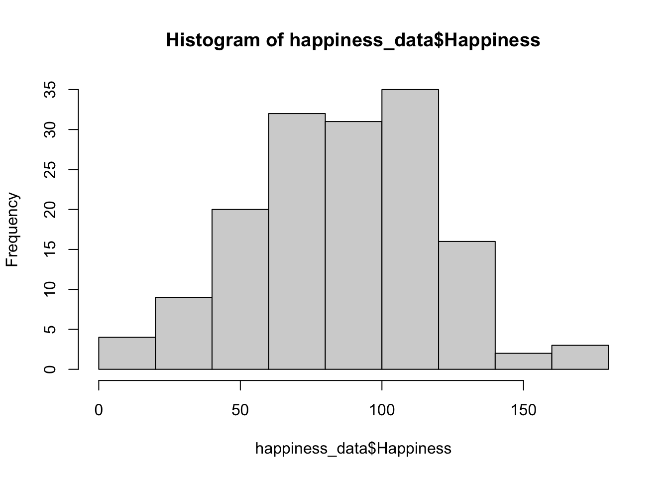
Alternatively, you can use ggplot2()
ggplot(happiness_data, aes(Happiness)) +
  geom_histogram(binwidth = 10, fill = "gray", color = "black")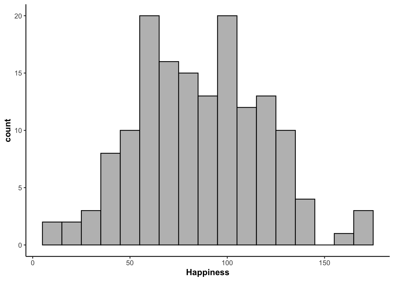
Correlation Tables
Regression models are based on the co-variation (or correlation) between variables. Therefore, we might want to first evaluate all of the pairwise correlations in the data.
The correlation package has a convenient function for creating a table of correlations that includes confidence intervals, t-values, df, and p.
happiness_data |>
  select(-Subject, -Type_of_Chocolate) |>
  correlation() |>
  select(-CI, -Method)
Or you can the correlation package to create a heat map
happiness_data |>
  select(-Subject, -Type_of_Chocolate) |>
  correlation() |>
  summary(redundant = TRUE) |>
  plot()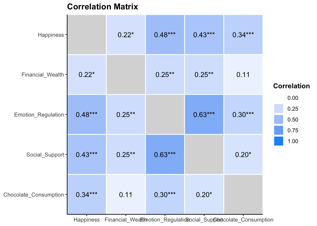
The sjPlot package has a convenient function for creating a correlation table/matrix
happiness_data |>
  select(-Subject, -Type_of_Chocolate) |>
tab_corr(na.deletion = "pairwise", digits = 2, triangle = "lower")| Happiness | Financial_Wealth | Emotion_Regulation | Social_Support | Chocolate_Consumption | |
| Happiness | |||||
| Financial_Wealth | 0.22** | ||||
| Emotion_Regulation | 0.48*** | 0.25** | |||
| Social_Support | 0.43*** | 0.25** | 0.63*** | ||
| Chocolate_Consumption | 0.34*** | 0.11 | 0.30*** | 0.20* | |
| Computed correlation used pearson-method with pairwise-deletion. | |||||
Scatterplots
Using the base R plot() function
plot(happiness_data$Financial_Wealth, happiness_data$Happiness)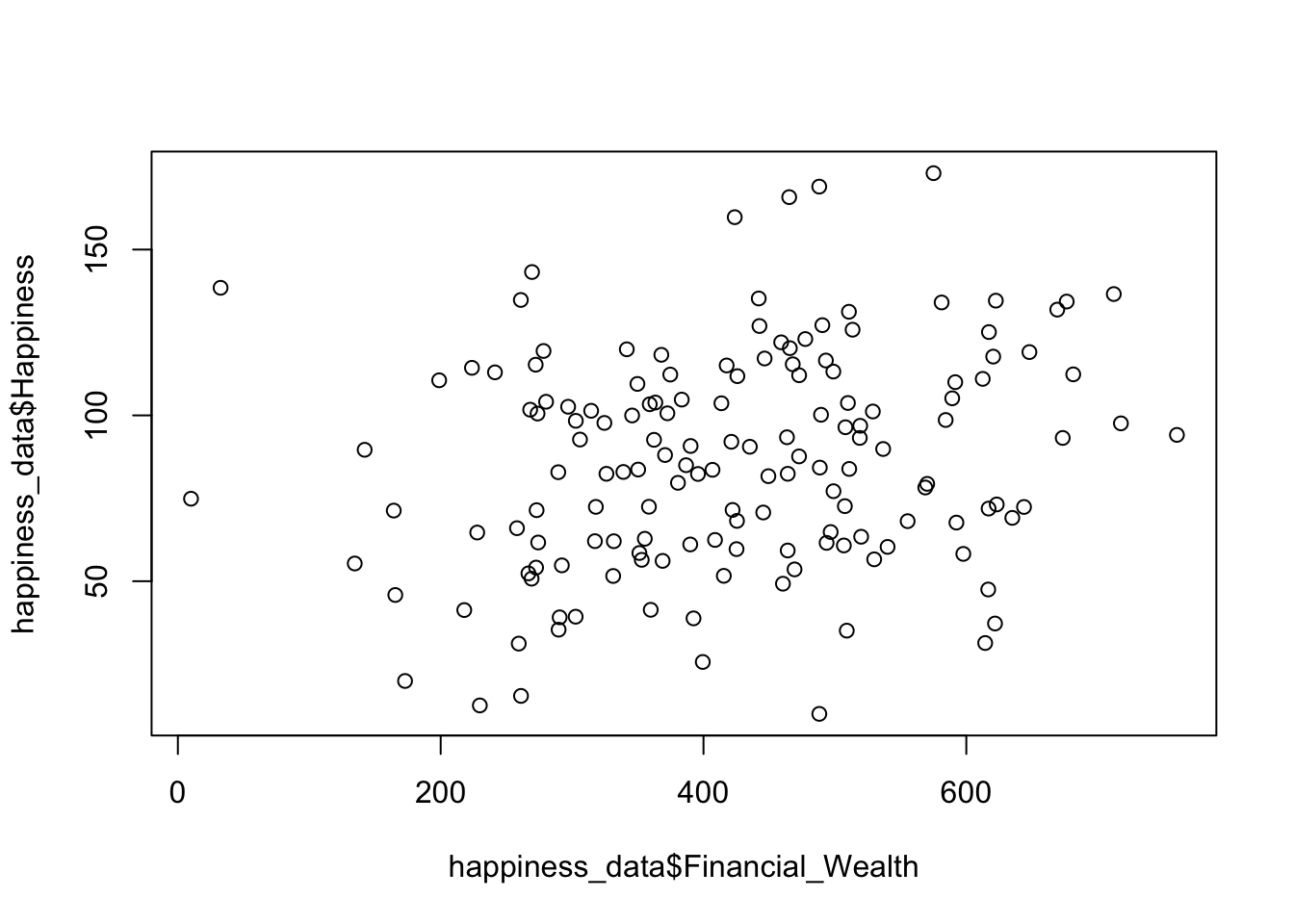
Using ggplot2
ggplot(happiness_data, aes(Financial_Wealth, Happiness)) +
  geom_point() +
  geom_smooth(method = "lm") +
  labs(x = "Financial Wealth (annual income)")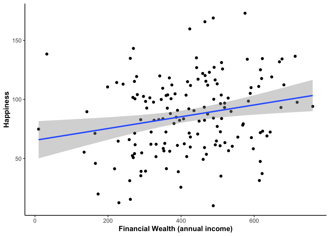
Using the correlation package
plot(cor_test(happiness_data, "Financial_Wealth", "Happiness"))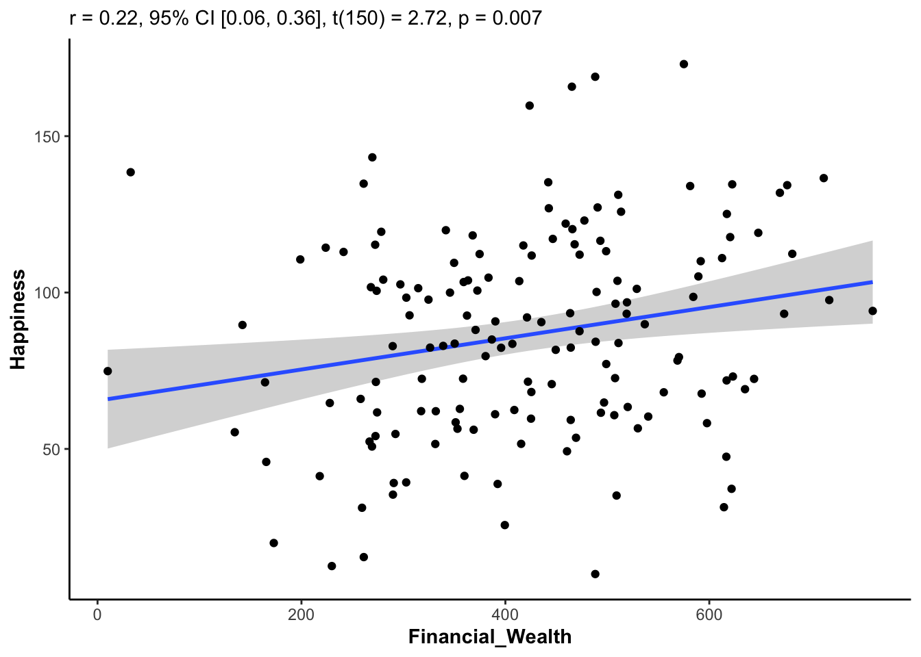
Regression
Regression models allow us to test more complicated relationships between variables. It is important to match your research question with the correct regression model. But also, thinking about the different types of regression models can help you clarify your research question. We will take a look at how to conduct the following regression models in R:
Simple regression
Multiple regression
Hierarchical regression
Mediation analysis
Moderation analysis
To conduct a regression model is fairly simple in R, all you need is to specify the regression formula in the lm() function.
Simple Regression
In what is called simple regression, there is only one predictor variable. Simple regression is not really necessary because it is directly equivalent to a correlation. However, it is useful to demonstrate what happens once you add multiple predictors into a model.
The formula in the lm() function takes on the form of: dv ~ iv.
Model
reg_simple <- lm(Happiness ~ Financial_Wealth, data = happiness_data)For regression models we can use the summary() call to print model results
summary(reg_simple)
Call:
lm(formula = Happiness ~ Financial_Wealth, data = happiness_data)

Residuals:
    Min      1Q  Median      3Q     Max
-79.766 -25.047   0.446  22.921  79.219

Coefficients:
                 Estimate Std. Error t value Pr(>|t|)
(Intercept)      65.41183    8.16488   8.011 2.93e-13 ***
Financial_Wealth  0.04989    0.01834   2.720  0.00729 **
---
Signif. codes:  0 '***' 0.001 '**' 0.01 '*' 0.05 '.' 0.1 ' ' 1

Residual standard error: 32.04 on 150 degrees of freedom
Multiple R-squared:  0.04701,   Adjusted R-squared:  0.04066
F-statistic:   7.4 on 1 and 150 DF,  p-value: 0.007293
The broom and performance packages provide an easy way to get model results into a table format
First using broom::glance() to get an overall model summary
glance(reg_simple)Then performance::model_parameters() to get unstandardized and standardized coefficient tables
model_parameters(reg_simple)model_parameters(reg_simple, standardize = "refit")My modeloutput package provides a way to display regression tables in output format similar to other statistical software packages like JASP or SPSS.
regression_tables(reg_simple)| Model Summary: Happiness | |||
|---|---|---|---|
| Model | R2 | R2 adj. | BIC |
| H1 | 0.047 | 0.041 | 1498.356 |
| H1: Happiness ~ Financial_Wealth; N = 152 | |||
| ANOVA Table: Happiness | ||||||
|---|---|---|---|---|---|---|
| Model | Term | Sum of Squares | df | Mean Square | F | p |
| H1 | Regression | 73472.006 | 2 | 36736.003 | 7.400 | 0.007 |
| H1 | Residual | 153960.370 | 150 | 1026.402 | ||
| H1: Happiness ~ Financial_Wealth; N = 152 | ||||||
| Regression Coefficients: Happiness | |||||||||
|---|---|---|---|---|---|---|---|---|---|
| Model | Term | Unstandardized | Standardized | t | df | p | |||
| b | 95% CI | β | 95% CI | SE | |||||
| H1 | (Intercept) | 65.412 | 49.279 — 81.545 | 0.000 | −0.157 — 0.157 | 0.079 | 8.011 | 150 | <0.001 |
| H1 | Financial_Wealth | 0.050 | 0.014 — 0.086 | 0.217 | 0.059 — 0.374 | 0.080 | 2.720 | 150 | 0.007 |
| H1: Happiness ~ Financial_Wealth; N = 152 | |||||||||
Multiple Regression
You can and will most likely want to include multiple predictor variables in a regression model. There will be a different interpretation of the beta coefficients compared to the simple regression model. Now, the beta coefficients will represent a unique contribution (controlling for all the other predictor variables) of that variable to the prediction of the dependent variable. We can compare the relative strengths of the beta coefficients to decide which variable(s) are the strongest predictors of the dependent variable.
In this case, we can go ahead and include all the continuous predictor variables in a model predicting Happiness and compare it with the simple regression when we only had Financial Wealth in the model.
Model
reg_multiple <- lm(Happiness ~ Financial_Wealth + Emotion_Regulation +
                     Social_Support + Chocolate_Consumption,
data = happiness_data)For regression models we can use the summary() call to print model results
summary(reg_multiple)
Call:
lm(formula = Happiness ~ Financial_Wealth + Emotion_Regulation +
    Social_Support + Chocolate_Consumption, data = happiness_data)

Residuals:
    Min      1Q  Median      3Q     Max
-75.847 -17.630  -0.047  17.125  66.950

Coefficients:
                      Estimate Std. Error t value Pr(>|t|)
(Intercept)           16.97620    9.73743   1.743  0.08336 .
Financial_Wealth       0.01778    0.01645   1.081  0.28162
Emotion_Regulation     0.46080    0.15209   3.030  0.00289 **
Social_Support         0.39466    0.17851   2.211  0.02859 *
Chocolate_Consumption  1.70732    0.59612   2.864  0.00480 **
---
Signif. codes:  0 '***' 0.001 '**' 0.01 '*' 0.05 '.' 0.1 ' ' 1

Residual standard error: 27.62 on 147 degrees of freedom
Multiple R-squared:  0.3061,    Adjusted R-squared:  0.2872
F-statistic: 16.21 on 4 and 147 DF,  p-value: 5.097e-11
The broom and performance packages provide an easy way to get model results into a table format
First using broom::glance() to get an overall model summary
glance(reg_multiple)Then performance::model_parameters() to get unstandardized and standardized coefficient tables
model_parameters(reg_multiple)model_parameters(reg_multiple, standardize = "refit")My modeloutput package provides a way to display regression tables in output format similar to other statistical software packages like JASP or SPSS.
regression_tables(reg_multiple)| Model Summary: Happiness | |||
|---|---|---|---|
| Model | R2 | R2 adj. | BIC |
| H1 | 0.306 | 0.287 | 1465.207 |
| H1: Happiness ~ Financial_Wealth + Emotion_Regulation + Social_Support + Chocolate_Consumption; N = 152 | |||
| ANOVA Table: Happiness | ||||||
|---|---|---|---|---|---|---|
| Model | Term | Sum of Squares | df | Mean Square | F | p |
| H1 | Regression | 20192.945 | 5 | 4038.589 | 16.210 | <0.001 |
| H1 | Residual | 112107.036 | 147 | 762.633 | ||
| H1: Happiness ~ Financial_Wealth + Emotion_Regulation + Social_Support + Chocolate_Consumption; N = 152 | ||||||
| Regression Coefficients: Happiness | |||||||||
|---|---|---|---|---|---|---|---|---|---|
| Model | Term | Unstandardized | Standardized | t | df | p | |||
| b | 95% CI | β | 95% CI | SE | |||||
| H1 | (Intercept) | 16.976 | −2.267 — 36.220 | 0.000 | −0.135 — 0.135 | 0.068 | 1.743 | 147 | 0.083 |
| H1 | Financial_Wealth | 0.018 | −0.015 — 0.050 | 0.077 | −0.064 — 0.219 | 0.071 | 1.081 | 147 | 0.282 |
| H1 | Emotion_Regulation | 0.461 | 0.160 — 0.761 | 0.277 | 0.096 — 0.458 | 0.092 | 3.030 | 147 | 0.003 |
| H1 | Social_Support | 0.395 | 0.042 — 0.747 | 0.197 | 0.021 — 0.373 | 0.089 | 2.211 | 147 | 0.029 |
| H1 | Chocolate_Consumption | 1.707 | 0.529 — 2.885 | 0.207 | 0.064 — 0.349 | 0.072 | 2.864 | 147 | 0.005 |
| H1: Happiness ~ Financial_Wealth + Emotion_Regulation + Social_Support + Chocolate_Consumption; N = 152 | |||||||||
Hierarchical Regression
Hierarchical regression is a multiptle regression approach where you compare multiple models with each other. We can compare the simple regression model we conducted above with only Financial_Wealth as a predictor of Happiness with the multiple regression model in which we added the other predictors.
We can use performance:compare_performance() to do model comparisons (hierarchical regression)
compare_performance(reg_simple, reg_multiple)In modeloutput::regression_tables() you can add up to three models to compare
regression_tables(reg_simple, reg_multiple)| Model Summary: Happiness | ||||||||||
|---|---|---|---|---|---|---|---|---|---|---|
| Model | R2 | R2 adj. | ΔR2 | ΔF | df1 | df2 | p | BIC | BF | P(Model|Data) |
| H1 | 0.047 | 0.041 | 1498.356 | |||||||
| H2 | 0.306 | 0.287 | 0.259 | 18.293 | 3 | 147 | <0.001 | 1465.207 | 1.58 × 10⁷ | 1.000 |
| H1: Happiness ~ Financial_Wealth; N = 152 | ||||||||||
| H2: Happiness ~ Financial_Wealth + Emotion_Regulation + Social_Support + Chocolate_Consumption; N = 152 | ||||||||||
| ANOVA Table: Happiness | ||||||
|---|---|---|---|---|---|---|
| Model | Term | Sum of Squares | df | Mean Square | F | p |
| H1 | Regression | 73472.006 | 2 | 36736.003 | 7.400 | 0.007 |
| H1 | Residual | 153960.370 | 150 | 1026.402 | ||
| H2 | Regression | 20192.945 | 5 | 4038.589 | 16.210 | <0.001 |
| H2 | Residual | 112107.036 | 147 | 762.633 | ||
| H1: Happiness ~ Financial_Wealth; N = 152 | ||||||
| H2: Happiness ~ Financial_Wealth + Emotion_Regulation + Social_Support + Chocolate_Consumption; N = 152 | ||||||
| Regression Coefficients: Happiness | |||||||||
|---|---|---|---|---|---|---|---|---|---|
| Model | Term | Unstandardized | Standardized | t | df | p | |||
| b | 95% CI | β | 95% CI | SE | |||||
| H1 | (Intercept) | 65.412 | 49.279 — 81.545 | 0.000 | −0.157 — 0.157 | 0.079 | 8.011 | 150 | <0.001 |
| H1 | Financial_Wealth | 0.050 | 0.014 — 0.086 | 0.217 | 0.059 — 0.374 | 0.080 | 2.720 | 150 | 0.007 |
| H2 | (Intercept) | 16.976 | −2.267 — 36.220 | 0.000 | −0.135 — 0.135 | 0.068 | 1.743 | 147 | 0.083 |
| H2 | Financial_Wealth | 0.018 | −0.015 — 0.050 | 0.077 | −0.064 — 0.219 | 0.071 | 1.081 | 147 | 0.282 |
| H2 | Emotion_Regulation | 0.461 | 0.160 — 0.761 | 0.277 | 0.096 — 0.458 | 0.092 | 3.030 | 147 | 0.003 |
| H2 | Social_Support | 0.395 | 0.042 — 0.747 | 0.197 | 0.021 — 0.373 | 0.089 | 2.211 | 147 | 0.029 |
| H2 | Chocolate_Consumption | 1.707 | 0.529 — 2.885 | 0.207 | 0.064 — 0.349 | 0.072 | 2.864 | 147 | 0.005 |
| H1: Happiness ~ Financial_Wealth; N = 152 | |||||||||
| H2: Happiness ~ Financial_Wealth + Emotion_Regulation + Social_Support + Chocolate_Consumption; N = 152 | |||||||||
Mediation
Mediation analysis allows us to test whether the effect of a predictor variable, on the dependent variable, “goes through” a mediator variable. This effect that “goes through” the mediator variable is called the indirect effect; whereas any effect of the predictor variable that does not “go through” the mediator is called the direct effect where:
Total Effect = Direct Effect + Indirect Effect
We are parsing the variance explained by the predictor variable into direct and indirect effects. Here are some possibilities for the outcome:
Full Mediation: The total effect of the predictor variable can be fully explained by the indirect effect. The mediator fully explains the effect of the predictor variable on the dependent variable. Direct effect = 0, indirect effect != 0.
Partial Mediation: The total effect of the predictor variable can be partially explained by the indirect effect. The mediator only partially explains the effect of the predictor variable on the dependent variable. Direct effect != 0, indirect effect != 0.
No Mediation: The total effect of the predictor variable can not be explained by the indirect effect; there is no indirect effect at all. Direct effect != 0, indirect effect = 0.
There are two general ways to perform a mediation analysis in R.
The standard regression method
Path analysis
Regression
The regression method requires multiple regression models because we have two dependent variables in the mode - the mediation and the outcome measure. The mediator acts as both an independent variable and dependent variable in the model. Because regression requires only one dependent variable, we cannot test the full model in one regression model. Instead, we have to test the different pieces of the model one at a time. We also need to perform a test on the indirect effect itself, which will require a separate model.
In order to evaluate the standardize coefficients (which is often times most useful), we need to first convert the the variables into z-scores. This is fairly straightforward but does require some extra code. A z-score is standardized score on the scale of standard deviation units and is calculated as:
z-score = (raw score - mean) / sd
We can create new columns representing the z-scores using mutate() from the dplyr package.
data_mediation <- happiness_data %>%
  mutate(Happiness_z =
           (Happiness - mean(Happiness)) / sd(Happiness),
         Social_Support_z =
           (Social_Support - mean(Social_Support)) / sd(Social_Support),
         Emotion_Regulation_z =
           (Emotion_Regulation - mean(Emotion_Regulation)) / sd(Emotion_Regulation))
The standard regression model typically involves three regression models and a model testing the indirect effect.
- A model with the total effect:
dv ~ iv
reg_total <- lm(Happiness_z ~ Social_Support_z,
data = data_mediation)- A model with the effect of the predictor on the mediator:
m ~ iv
reg_med <- lm(Emotion_Regulation_z ~ Social_Support_z,
data = data_mediation)- A model with the direct effect and the effect of the mediator:
dv ~ iv + m
reg_direct <- lm(Happiness_z ~ Emotion_Regulation_z + Social_Support_z,
data = data_mediation)- A statistical test of the indirect effect:
mediation::mediate()
model_mediation <- mediation::mediate(reg_med, reg_direct,
                                      treat = "Social_Support_z",
                                      mediator = "Emotion_Regulation_z",
                                      boot = TRUE, sims = 1000,
boot.ci.type = "bca")1. DV ~ IV
glance(reg_total)model_parameters(reg_total, standardize = "refit")2. M ~ IV
glance(reg_med)model_parameters(reg_med, standardize = "refit")3. DV ~ IV + M
glance(reg_direct)model_parameters(reg_direct, standardize = "refit")4. Mediation
model_parameters(model_mediation)Regression Tables
regression_tables(reg_total, reg_direct)| Model Summary: Happiness_z | ||||||||||
|---|---|---|---|---|---|---|---|---|---|---|
| Model | R2 | R2 adj. | ΔR2 | ΔF | df1 | df2 | p | BIC | BF | P(Model|Data) |
| H1 | 0.187 | 0.181 | 413.995 | |||||||
| H2 | 0.261 | 0.251 | 0.074 | 14.944 | 1 | 149 | <0.001 | 404.491 | 1.16 × 10² | 0.991 |
| H1: Happiness_z ~ Social_Support_z; N = 152 | ||||||||||
| H2: Happiness_z ~ Emotion_Regulation_z + Social_Support_z; N = 152 | ||||||||||
| ANOVA Table: Happiness_z | ||||||
|---|---|---|---|---|---|---|
| Model | Term | Sum of Squares | df | Mean Square | F | p |
| H1 | Regression | 28.207 | 2 | 14.103 | 34.456 | <0.001 |
| H1 | Residual | 122.793 | 150 | 0.819 | ||
| H2 | Regression | 15.276 | 3 | 5.092 | 26.302 | <0.001 |
| H2 | Residual | 111.600 | 149 | 0.749 | ||
| H1: Happiness_z ~ Social_Support_z; N = 152 | ||||||
| H2: Happiness_z ~ Emotion_Regulation_z + Social_Support_z; N = 152 | ||||||
| Regression Coefficients: Happiness_z | |||||||||
|---|---|---|---|---|---|---|---|---|---|
| Model | Term | Unstandardized | Standardized | t | df | p | |||
| b | 95% CI | β | 95% CI | SE | |||||
| H1 | (Intercept) | 0.000 | −0.145 — 0.145 | 0.000 | −0.145 — 0.145 | 0.073 | 0.000 | 150 | 1.000 |
| H1 | Social_Support_z | 0.432 | 0.287 — 0.578 | 0.432 | 0.287 — 0.578 | 0.074 | 5.870 | 150 | <0.001 |
| H2 | (Intercept) | 0.000 | −0.139 — 0.139 | 0.000 | −0.139 — 0.139 | 0.070 | 0.000 | 149 | 1.000 |
| H2 | Emotion_Regulation_z | 0.350 | 0.171 — 0.530 | 0.350 | 0.171 — 0.530 | 0.091 | 3.866 | 149 | <0.001 |
| H2 | Social_Support_z | 0.212 | 0.033 — 0.391 | 0.212 | 0.033 — 0.391 | 0.091 | 2.335 | 149 | 0.021 |
| H1: Happiness_z ~ Social_Support_z; N = 152 | |||||||||
| H2: Happiness_z ~ Emotion_Regulation_z + Social_Support_z; N = 152 | |||||||||
regression_tables(reg_med)| Model Summary: Emotion_Regulation_z | |||
|---|---|---|---|
| Model | R2 | R2 adj. | BIC |
| H1 | 0.396 | 0.392 | 368.722 |
| H1: Emotion_Regulation_z ~ Social_Support_z; N = 152 | |||
| ANOVA Table: Emotion_Regulation_z | ||||||
|---|---|---|---|---|---|---|
| Model | Term | Sum of Squares | df | Mean Square | F | p |
| H1 | Regression | 59.837 | 2 | 29.918 | 98.456 | <0.001 |
| H1 | Residual | 91.163 | 150 | 0.608 | ||
| H1: Emotion_Regulation_z ~ Social_Support_z; N = 152 | ||||||
| Regression Coefficients: Emotion_Regulation_z | |||||||||
|---|---|---|---|---|---|---|---|---|---|
| Model | Term | Unstandardized | Standardized | t | df | p | |||
| b | 95% CI | β | 95% CI | SE | |||||
| H1 | (Intercept) | 0.000 | −0.125 — 0.125 | 0.000 | −0.125 — 0.125 | 0.063 | 0.000 | 150 | 1.000 |
| H1 | Social_Support_z | 0.630 | 0.504 — 0.755 | 0.630 | 0.504 — 0.755 | 0.063 | 9.922 | 150 | <0.001 |
| H1: Emotion_Regulation_z ~ Social_Support_z; N = 152 | |||||||||
Mediation
model_parameters(model_mediation)Path Analysis
There is a statistical modelling approach called path analysis that does allow for multiple dependent variables in a single model. Here is how to specify a path analysis model using the lavaan package.
See the lavaan website for how to conduct mediation in lavaan
Model
model <- "
# a path
Emotion_Regulation ~ a*Social_Support

# b path
Happiness ~ b*Emotion_Regulation

# c prime path
Happiness ~ c*Social_Support

# indirect and total effects
indirect := a*b
total := c + a*b
"

fit <- sem(model, data = happiness_data)summary(fit, standardized = TRUE)lavaan 0.6.16 ended normally after 1 iteration
Estimator ML
Optimization method NLMINB
Number of model parameters 5
Number of observations 152
Model Test User Model:
Test statistic 0.000
Degrees of freedom 0
Parameter Estimates:
Standard errors Standard
Information Expected
Information saturated (h1) model Structured
Regressions:
Estimate Std.Err z-value P(>|z|) Std.lv Std.all
Emotion_Regulation ~
Socl_Spprt (a) 0.760 0.076 9.988 0.000 0.760 0.629
Happiness ~
Emtn_Rgltn (b) 0.582 0.149 3.905 0.000 0.582 0.350
Socl_Spprt (c) 0.424 0.180 2.358 0.018 0.424 0.212
Variances:
Estimate Std.Err z-value P(>|z|) Std.lv Std.all
.Emotion_Regltn 232.557 26.676 8.718 0.000 232.557 0.604
.Happiness 785.537 90.107 8.718 0.000 785.537 0.739
Defined Parameters:
Estimate Std.Err z-value P(>|z|) Std.lv Std.all
indirect 0.442 0.122 3.637 0.000 0.442 0.221
total 0.866 0.147 5.909 0.000 0.866 0.432I also have a package, semoutput for displaying results from lavaan models:
sem_tables(fit)| Model Significance | |||
| N | χ2 | df | p |
|---|---|---|---|
| 152 | 0.000 | 0 | |
| Model Fit | ||||||
| CFI | RMSEA | 90% CI | TLI | SRMR | AIC | BIC |
|---|---|---|---|---|---|---|
| 1.000 | 0.000 | 0.000 — 0.000 | 1.000 | 0.000 | 2714.271 | 2729.391 |
| Regression Paths | |||||||
| Predictor | DV | Standardized | |||||
|---|---|---|---|---|---|---|---|
| β | 95% CI | sig | SE | z | p | ||
| Social_Support | Emotion_Regulation | 0.629 | 0.544 — 0.715 | *** | 0.044 | 14.356 | 0.000 |
| Emotion_Regulation | Happiness | 0.350 | 0.181 — 0.520 | *** | 0.086 | 4.057 | <0.001 |
| Social_Support | Happiness | 0.212 | 0.039 — 0.384 | * | 0.088 | 2.402 | 0.016 |
| a*b | indirect | 0.221 | 0.109 — 0.333 | *** | 0.057 | 3.859 | <0.001 |
| c+a*b | total | 0.432 | 0.309 — 0.555 | *** | 0.063 | 6.882 | <0.001 |
| * p < .05; ** p < .01; *** p < .001 | |||||||
size <- .65
semPaths(fit, whatLabels = "std", layout = "tree2",
         rotation = 2, style = "lisrel", optimizeLatRes = TRUE,
         structural = FALSE, layoutSplit = FALSE,
         intercepts = FALSE, residuals = FALSE,
         curve = 1, curvature = 3, nCharNodes = 8,
         sizeLat = 11 * size, sizeMan = 11 * size, sizeMan2 = 4 * size,
         edge.label.cex = 1.2 * size,
         edge.color = "#000000", edge.label.position = .40)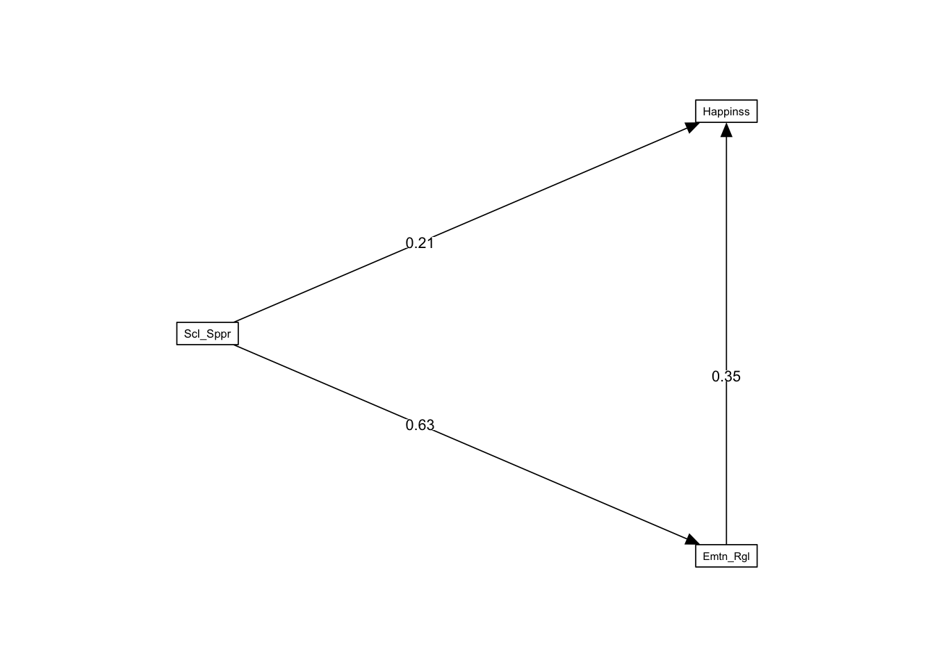
It is highly advised to calculate bootstrapped and bias-corrected confidence intervals around the indirect effect:
monteCarloCI(fit, nRep = 1000, standardized = TRUE)Moderation
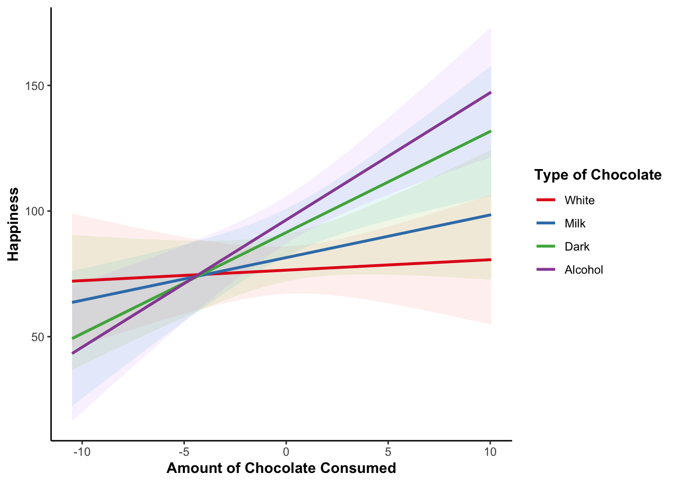
Another type of multiple regression model is the moderation analysis. The concept of moderation in regression is analogous to the concept of an interaction in ANOVA. The idea here is that the relationship (correlation or slope) between two variables changes as a function of another variable, called the moderator. As the values on the moderator variable increases, the correlation or slope might increase or decrease. The moderator can be either continuous or categorical.
In our happiness data, we can test whether the relationship between chocolate consumption and happiness is moderated by the type of chocolate consumed. In this case, type of chocolate is a categorical variable: White, milk, dark, or alcohol.
It is highly advisable to first “center” the predictor and moderator variables. Centering refers to centering the scores around the mean (making the mean = 0). This can simply be done by subtracting out the mean from each score. We can do this with mutate() from the dplyr package.
Since type of chocolate is categorical we do not need to center it.
data_mod <- happiness_data %>%
  mutate(Chocolate_Consumed_c =
           Chocolate_Consumption - mean(Chocolate_Consumption))
Model
model_null <- lm(Happiness ~ Chocolate_Consumed_c + Type_of_Chocolate,
                 data = data_mod)

model_moderation <- lm(Happiness ~ Chocolate_Consumed_c * Type_of_Chocolate,
data = data_mod)summary(model_null)
Call:
lm(formula = Happiness ~ Chocolate_Consumed_c + Type_of_Chocolate,
    data = data_mod)

Residuals:
    Min      1Q  Median      3Q     Max
-81.628 -17.038  -0.842  20.550  72.419

Coefficients:
                         Estimate Std. Error t value Pr(>|t|)
(Intercept)               76.4680     4.8883  15.643  < 2e-16 ***
Chocolate_Consumed_c       2.8006     0.6192   4.523 1.25e-05 ***
Type_of_ChocolateMilk      5.0000     6.9132   0.723   0.4707
Type_of_ChocolateDark     15.0000     6.9132   2.170   0.0316 *
Type_of_ChocolateAlcohol  20.0000     6.9132   2.893   0.0044 **
---
Signif. codes:  0 '***' 0.001 '**' 0.01 '*' 0.05 '.' 0.1 ' ' 1

Residual standard error: 30.13 on 147 degrees of freedom
Multiple R-squared:  0.1738,    Adjusted R-squared:  0.1513
F-statistic: 7.729 on 4 and 147 DF, p-value: 1.111e-05summary(model_moderation)
Call:
lm(formula = Happiness ~ Chocolate_Consumed_c * Type_of_Chocolate,
    data = data_mod)

Residuals:
   Min     1Q Median     3Q    Max
-68.72 -18.19  -2.37  20.53  74.22

Coefficients:
                                              Estimate Std. Error t value
(Intercept)                                    76.4680     4.7887  15.968
Chocolate_Consumed_c                            0.4167     1.2132   0.343
Type_of_ChocolateMilk                           5.0000     6.7722   0.738
Type_of_ChocolateDark                          15.0000     6.7722   2.215
Type_of_ChocolateAlcohol                       20.0000     6.7722   2.953
Chocolate_Consumed_c:Type_of_ChocolateMilk      1.2821     1.7158   0.747
Chocolate_Consumed_c:Type_of_ChocolateDark      3.6060     1.7158   2.102
Chocolate_Consumed_c:Type_of_ChocolateAlcohol   4.6477     1.7158   2.709
                                              Pr(>|t|)
(Intercept)                                    < 2e-16 ***
Chocolate_Consumed_c                           0.73176
Type_of_ChocolateMilk                          0.46153
Type_of_ChocolateDark                          0.02834 *
Type_of_ChocolateAlcohol                       0.00367 **
Chocolate_Consumed_c:Type_of_ChocolateMilk     0.45613
Chocolate_Consumed_c:Type_of_ChocolateDark     0.03733 *
Chocolate_Consumed_c:Type_of_ChocolateAlcohol  0.00757 **
---
Signif. codes:  0 '***' 0.001 '**' 0.01 '*' 0.05 '.' 0.1 ' ' 1

Residual standard error: 29.52 on 144 degrees of freedom
Multiple R-squared:  0.2233,    Adjusted R-squared:  0.1855
F-statistic: 5.914 on 7 and 144 DF,  p-value: 4.684e-06
Null Model
glance(model_null)model_parameters(model_null, standardize = "refit")Interaction
glance(model_moderation)model_parameters(model_moderation, standardize = "refit")regression_tables(model_null, model_moderation)| Model Summary: Happiness | ||||||||||
|---|---|---|---|---|---|---|---|---|---|---|
| Model | R2 | R2 adj. | ΔR2 | ΔF | df1 | df2 | p | BIC | BF | P(Model|Data) |
| H1 | 0.174 | 0.151 | 1491.733 | |||||||
| H2 | 0.223 | 0.186 | 0.050 | 3.061 | 3 | 144 | 0.030 | 1497.409 | 5.85 × 10⁻² | 0.055 |
| H1: Happiness ~ Chocolate_Consumed_c + Type_of_Chocolate; N = 152 | ||||||||||
| H2: Happiness ~ Chocolate_Consumed_c * Type_of_Chocolate; N = 152 | ||||||||||
| ANOVA Table: Happiness | ||||||
|---|---|---|---|---|---|---|
| Model | Term | Sum of Squares | df | Mean Square | F | p |
| H1 | Regression | 250273.269 | 5 | 50054.654 | 7.729 | <0.001 |
| H1 | Residual | 133482.237 | 147 | 908.042 | ||
| H2 | Regression | 239803.383 | 8 | 29975.423 | 5.914 | <0.001 |
| H2 | Residual | 125481.246 | 144 | 871.398 | ||
| H1: Happiness ~ Chocolate_Consumed_c + Type_of_Chocolate; N = 152 | ||||||
| H2: Happiness ~ Chocolate_Consumed_c * Type_of_Chocolate; N = 152 | ||||||
| Regression Coefficients: Happiness | |||||||||
|---|---|---|---|---|---|---|---|---|---|
| Model | Term | Unstandardized | Standardized | t | df | p | |||
| b | 95% CI | β | 95% CI | SE | |||||
| H1 | (Intercept) | 76.468 | 66.808 — 86.129 | −0.306 | −0.601 — −0.010 | 0.149 | 15.643 | 147 | <0.001 |
| H1 | Chocolate_Consumed_c | 2.801 | 1.577 — 4.024 | 0.339 | 0.191 — 0.487 | 0.075 | 4.523 | 147 | <0.001 |
| H1 | Type_of_ChocolateMilk | 5.000 | −8.662 — 18.662 | 0.153 | −0.265 — 0.571 | 0.211 | 0.723 | 147 | 0.471 |
| H1 | Type_of_ChocolateDark | 15.000 | 1.338 — 28.662 | 0.459 | 0.041 — 0.876 | 0.211 | 2.170 | 147 | 0.032 |
| H1 | Type_of_ChocolateAlcohol | 20.000 | 6.338 — 33.662 | 0.611 | 0.194 — 1.029 | 0.211 | 2.893 | 147 | 0.004 |
| H2 | (Intercept) | 76.468 | 67.003 — 85.933 | −0.306 | −0.595 — −0.016 | 0.146 | 15.968 | 144 | <0.001 |
| H2 | Chocolate_Consumed_c | 0.417 | −1.981 — 2.815 | 0.050 | −0.240 — 0.341 | 0.147 | 0.343 | 144 | 0.732 |
| H2 | Type_of_ChocolateMilk | 5.000 | −8.386 — 18.386 | 0.153 | −0.256 — 0.562 | 0.207 | 0.738 | 144 | 0.462 |
| H2 | Type_of_ChocolateDark | 15.000 | 1.614 — 28.386 | 0.459 | 0.049 — 0.868 | 0.207 | 2.215 | 144 | 0.028 |
| H2 | Type_of_ChocolateAlcohol | 20.000 | 6.614 — 33.386 | 0.611 | 0.202 — 1.021 | 0.207 | 2.953 | 144 | 0.004 |
| H2 | Chocolate_Consumed_c:Type_of_ChocolateMilk | 1.282 | −2.109 — 4.673 | 0.155 | −0.255 — 0.566 | 0.208 | 0.747 | 144 | 0.456 |
| H2 | Chocolate_Consumed_c:Type_of_ChocolateDark | 3.606 | 0.215 — 6.997 | 0.437 | 0.026 — 0.847 | 0.208 | 2.102 | 144 | 0.037 |
| H2 | Chocolate_Consumed_c:Type_of_ChocolateAlcohol | 4.648 | 1.256 — 8.039 | 0.563 | 0.152 — 0.973 | 0.208 | 2.709 | 144 | 0.008 |
| H1: Happiness ~ Chocolate_Consumed_c + Type_of_Chocolate; N = 152 | |||||||||
| H2: Happiness ~ Chocolate_Consumed_c * Type_of_Chocolate; N = 152 | |||||||||
To better understand the nature of a moderation, it helps to plot the results.
The easiest way to plot the results of a moderation analysis is using the plot_model() function from the sjPlot package. Note that it is a bit more complicated to plot a moderation analysis when the moderator is a continuous variable instead of categorical but the sjPlot package actually makes it a bit easier.
plot_model(model_moderation, typ = "int")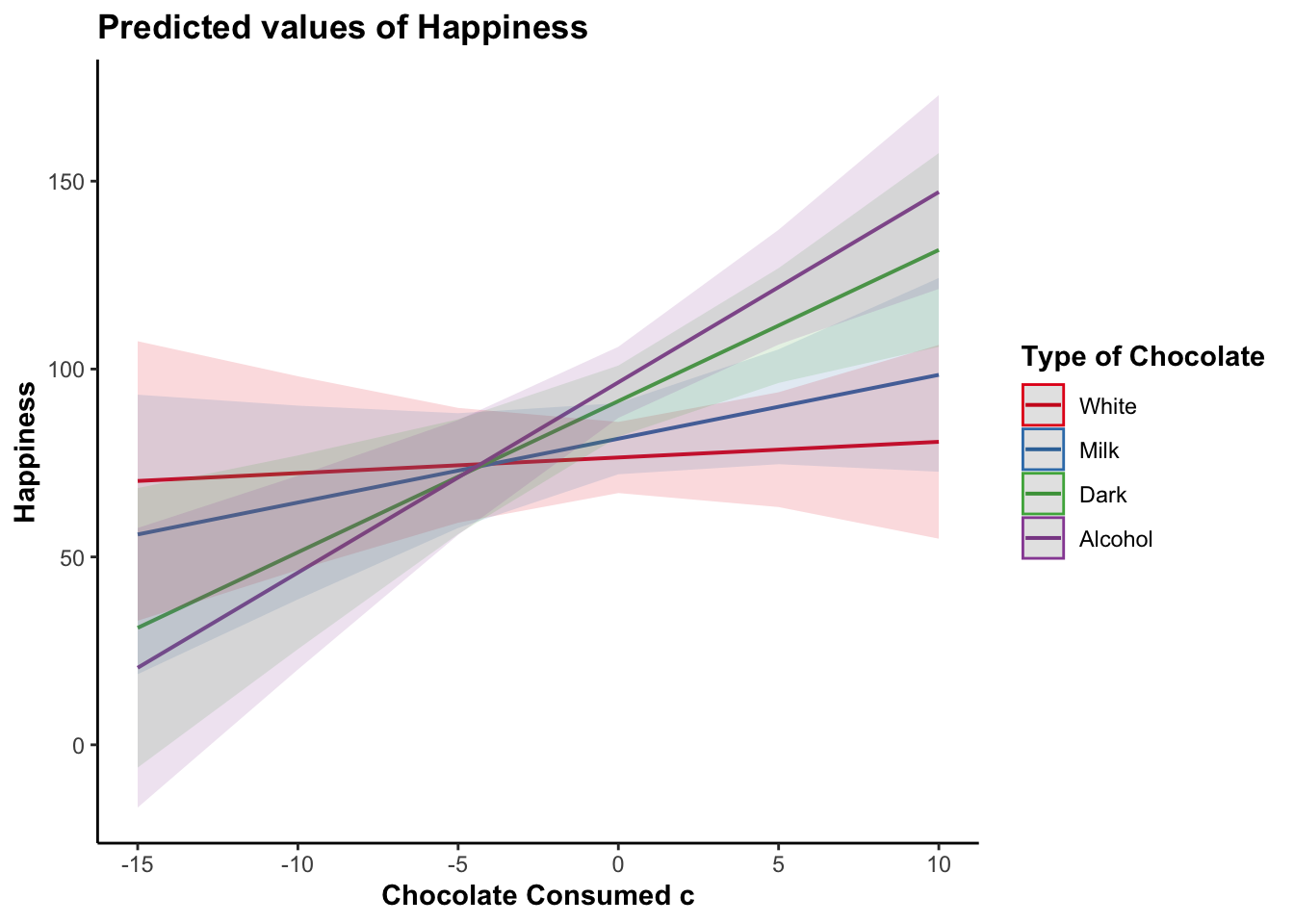
The most customizable way to plot model results is using the ggeffects and ggplot2 packages. We can use ggeffect() to get a data frame with estimated model values for specified terms in the model and the dependent variable.
For continuous variables, we can customize at what values we want to plot. For “all” possible values from the original data we can specify [all]. If your variable was standardized before entering it into the model you can use [2, 0, -2] to get values at +2 standard deviations above the mean, the mean, and -2 standard deviations below the mean.
data_plot <- ggeffect(model_moderation,
                       terms = c("Chocolate_Consumed_c [all]",
                                 "Type_of_Chocolate")) |>
  rename(Chocolate_Consumed_c = x, Type_of_Chocolate = group,
Happiness = predicted)ggplot(data_plot, aes(Chocolate_Consumed_c, Happiness,
color = Type_of_Chocolate)) +
geom_ribbon(aes(ymin = conf.low, ymax = conf.high,
fill = Type_of_Chocolate),
show.legend = FALSE, alpha = .1, color = NA) +
geom_smooth(method = "lm", alpha = 0) +
scale_color_brewer(palette = "Set1",
guide_legend(title = "Type of Chocolate")) +
labs(x = "Amount of Chocolate Consumed")