data <- data.frame(x = c(1,6,4,3,7,5,8,4),
                   y = c(2,3,2,1,4,6,4,3))

y_mean <- mean(data$y)Data Transformation
Class 3
The main objective of this class is to get familiar with the basic functions in dplyr for performing basic data transformations.
🖥️ Slides
Prepare
Before starting this class:
📦 Install the gt package
Download sample data files:
⬇️ class_3_repetition_rawdata.txt
⬇️ class_3_mnemonic_rawdata.csv
This is The Way
Although you will be learning R in this class, it might be more appropriate to say that you are learning the tidyverse.

The tidyverse is a set of packages that share an underlying design philosophy, grammar, and data structures. The tidyverse consists of packages that are simple and intuitive to use and will take you from importing data (with readr), restructuring and transforming data (with tidyr and dplyr), and to graphically visualizing data (with ggplot2).
dplyr
The language of dplyr will be the underlying framework for how you will think about manipulating and transforming data in R.
![]()
dplyr uses intuitive language that you are already familiar with. As with any R function, you can think of functions in the dplyr package as verbs that refer to performing a particular action on a data frame.
rename()renames columnsfilter()filters rows based on their values in specified columnsselect()selects (or removes) columnsmutate()creates new columns based on transformation from other columns, or edits values within existing columnssummarise()aggregates across rows to create a summary statistic (means, standard deviations, etc.)
For more information on these functions Visit the dplyr webpage
For more detailed instructions on how to use the dplyr functions see the Data Transformation chapter in the popular R for Data Science book.
Stay within the Data Frame
Not only is the language of dplyr intuitive but it allows you to perform data manipulations all within the data frame itself, without having to create external variables, lists, for loops, etc.
It can be tempting to hold information outside of a data frame but in general I suggest avoiding this strategy. Instead, hold the information in a new column within the data frame itself.
For example: A common strategy I see in many R scripts is to hold the mean or count of a column of values outside the data frame and in a new variable in the Environment.
This variable is then used to subtract out the mean from the values in column y
library(dplyr)

data <- mutate(data,
y_new = y - y_mean)| x | y | y_new |
|---|---|---|
| 1.000 | 2.000 | −1.125 |
| 6.000 | 3.000 | −0.125 |
| 4.000 | 2.000 | −1.125 |
| 3.000 | 1.000 | −2.125 |
| 7.000 | 4.000 | 0.875 |
| 5.000 | 6.000 | 2.875 |
Although there is nothing wrong with this approach, in general, I would advise against this strategy.
A better strategy is to do all this without leaving the data frame data.
library(dplyr)

data <- data.frame(x = c(1,6,4,3,7,5,8,4),
                   y = c(2,3,2,1,4,6,4,3))

data <- mutate(data,
               y_mean = mean(y),
y_new = y - y_mean)| x | y | y_mean | y_new |
|---|---|---|---|
| 1.000 | 2.000 | 3.125 | −1.125 |
| 6.000 | 3.000 | 3.125 | −0.125 |
| 4.000 | 2.000 | 3.125 | −1.125 |
| 3.000 | 1.000 | 3.125 | −2.125 |
| 7.000 | 4.000 | 3.125 | 0.875 |
| 5.000 | 6.000 | 3.125 | 2.875 |
Example Data Set
Let’s use what we learned in Class2 and import two data files.
⬇️ class_3_repetition_rawdata.txt
⬇️ class_3_mnemonic_rawdata.csv
Try to figure out how to import the data yourself (hint: use the Import Datatset GUI to help identify the correct file path and import parameters)
Show the Code
library(readr)

repetition_import <- read_delim("data/class_3_repetition_rawdata.txt",
                                delim = "\t", escape_double = FALSE,
                                trim_ws = TRUE)

mnemonic_import <- read_csv("data/class_3_mnemonic_rawdata.csv")
These data come from a hypothetical (I made it up) research study to compare the effectiveness of two memory techniques, a mnemonic technique and a spaced repetition technique, for improving memory retention. Participants were randomly assigned to one of the two memory techniques and completed 3 memory tests (A, B, and C). The number of correctly recalled words for each memory test was recorded in the two data files by research assistants.
Use what you learned from Class 1 to explore the data
what are the column names?
what type of values are in each column?
You will recognize there are some differences between these two data sets even though they both contain memory recall performance on 3 memory tests (A, B, and C). It turns out that the research assistant who ran participants in the spaced repetition condition did not follow the lab’s protocol for recording data 🤦♀️
They used wrong column names, recorded the memory tests as X, Y, and Z (A, B, and C, respectively), they left out what condition these data were from, and they gave some particpants less than 3 memory tests! 🤬
rename()
First, let’s fix the RA’s mistake by renaming the columns in the spaced repetition data as they are named in the mnemonic data. We can do so using the rename() function. The format for this function looks something like:
rename(new_name = old_name)Here is how we would rename the columns in the spaced repetition data we imported.
library(dplyr)

repetition_data <- repetition_import |>
  rename(participant_id = `subject number`,
         word_list = List,
         recall_correct = recallCorrect)
For more options on how to use rename() see the documentation here
filter()
filter() is an inclusive filter and requires the use of logical statements. Here are a list of some commone logical operators in R:
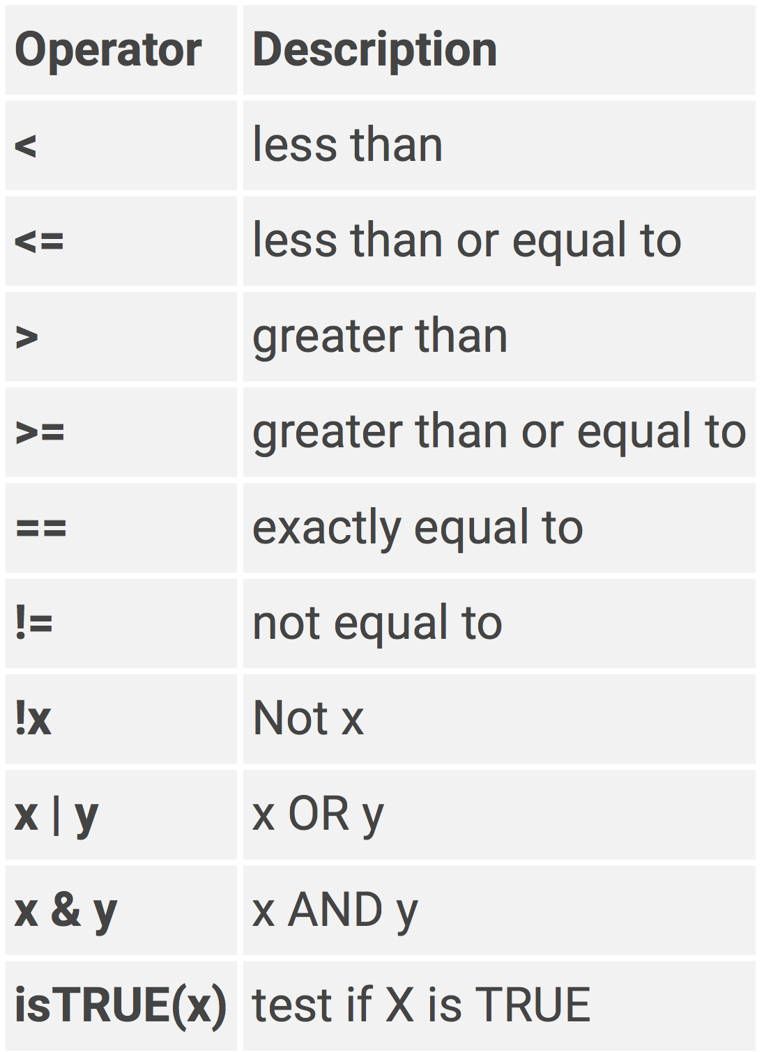
In addition to the logical operators, other functions can be used in filter(), such as:
is.na()- include if missing!is.na()- include if not missingbetween()- values that are between a certain range of numbersnear()- values that are near a certain value
For more options on how to use filter() see the documentation here.
Let’s remove rows that correspond to those participants that did not complete 3 memory tests. It turns out that those participants were always ran on Thursday or Friday, must have been a bad day for the research assistant 😢. We can use filter() to remove rows that have Thursday or Friday in the day column.
repetition_data <- repetition_data |>
  filter(day != "Thursday", day != "Friday")
select()
select() allows you to select which columns to keep and/or remove.
select(columns, to, keep)select(-columns, -to, -remove)select() can be used with more complex operators and tidyselect functions, see the documentation here.
For the repetition data, let’s only keep the following columns
participant_id
word_list
recall_correct
repetition_data <- repetition_data |>
  select(participant_id, word_list, recall_correct)
Another way to do this would be:
repetition_data <- repetition_data |>
  select(-day, -time, -computer_station)
mutate()
mutate() is a very powerful function. It basically allows you to do any computation or transformation on the values in the data frame. See the full documentation here.
The basic format for mutate goes something like:
mutate(column_name = value,
       another_col = a_function(),
       last_col = col1 + col2)
Within mutate() the = sign functions similarly to the assignment operator <-, where the result of whatever is on the right-hand side of = gets assigned to the column that is specified on the left-hand side (an existing column or a new one you are creating).
I want to demonstrate basic but common examples of using mutate()
We need to create a column specifying what condition the spaced repetition data came from, dang RA!
repetition_data <- repetition_data |>
  mutate(condition = "spaced repetition")
Easy!
Now let’s do something a little more complicated.
case_when()
case_when() is basically a sequence of if else type of statements where each statement is evaluated, if it is true then it is given a certain value, else the next statement is evaluated, and so on. The basic format of case_when() looks like:
mutate(a_column = case_when(a logical statement ~ a value,
                            another statement ~ another value,
                            .default = and another value))
Let’s see an example of this with the spaced repetition data. We need to change the values in the word_list column so that X is A, Y is B, and Z is C.
repetition_data <- repetition_data |>
  mutate(word_list = case_when(word_list == "X" ~ "A",
                               word_list == "Y" ~ "B",
                               word_list == "Z" ~ "C"))
Just to be clear, you can create an entirely new column this way
repetition_data <- repetition_data |>
  mutate(new_word_list = case_when(word_list == "X" ~ "A",
                                   word_list == "Y" ~ "B",
                                   word_list == "Z" ~ "C"))
.by =
This next computation is not necessary for our example data set but I want to demonstrate the use of mutate(.by = ). This option is very handy if you want to perform functions separately on different groups or splits of the data frame.
For example, let’s calculate the mean for each word list separately.
repetition_data <- repetition_data |>
  mutate(.by = word_list,
         word_list_mean = mean(recall_correct))
Compare this with
repetition_data <- repetition_data |>
  mutate(word_list_mean = mean(recall_correct))
You can use multiple columns in .by =
repetition_data <- repetition_data |>
  mutate(.by = c(participant_id, word_list),
         word_list_mean = mean(recall_correct))
It doesn’t make much sense in this case
The .by = option becomes extremely useful when used in summarise() which we will get to in a bit.
rowwise()
While .by = is used when performing functions on groups of rows, rowwise() is used when you want to perform operations row by row, treating each row as a single group. This is useful when you want to aggregate data (e.g., mean()) across multiple columns.
The data set we are working with does not provide a good demonstration of this so let’s create a different set of data to look at how to use rowwise()
data_sample <- data.frame(ID = 1:5,
                          Q1 = sample(1:50, 5),
                          Q2 = sample(1:50, 5),
Q3 = sample(1:50, 5))| ID | Q1 | Q2 | Q3 |
|---|---|---|---|
| 1.000 | 43.000 | 34.000 | 42.000 |
| 2.000 | 4.000 | 28.000 | 34.000 |
| 3.000 | 13.000 | 15.000 | 20.000 |
| 4.000 | 49.000 | 25.000 | 50.000 |
| 5.000 | 18.000 | 41.000 | 2.000 |
Here is an example where we have a single row per participant with columns representing their responses to three different questions. Let’s say we want to calculate their mean response across these three columns.
Important
You NEED to ungroup() the data frame whenever you are done with rowwise()
data_sample <- data_sample |>
  rowwise() |>
  mutate(Q_mean = mean(c(Q1, Q2, Q3))) |>
ungroup()| ID | Q1 | Q2 | Q3 | Q_mean |
|---|---|---|---|---|
| 1.000 | 43.000 | 34.000 | 42.000 | 39.667 |
| 2.000 | 4.000 | 28.000 | 34.000 | 22.000 |
| 3.000 | 13.000 | 15.000 | 20.000 | 16.000 |
| 4.000 | 49.000 | 25.000 | 50.000 | 41.333 |
| 5.000 | 18.000 | 41.000 | 2.000 | 20.333 |
Note the difference when you don’t use rowwise(), it calculates the mean across all rows in the data
data_sample <- data_sample |>
mutate(Q_mean = mean(c(Q1, Q2, Q3)))| ID | Q1 | Q2 | Q3 | Q_mean |
|---|---|---|---|---|
| 1.000 | 43.000 | 34.000 | 42.000 | 27.867 |
| 2.000 | 4.000 | 28.000 | 34.000 | 27.867 |
| 3.000 | 13.000 | 15.000 | 20.000 | 27.867 |
| 4.000 | 49.000 | 25.000 | 50.000 | 27.867 |
| 5.000 | 18.000 | 41.000 | 2.000 | 27.867 |
We can put all the dplyr functions together through a series of pipes:
repetition_data <- repetition_import |>
  rename(participant_id = `subject number`,
         word_list = List,
         recall_correct = recallCorrect) |>
  filter(day != "Thursday", day != "Friday") |>
  select(participant_id, word_list, recall_correct) |>
  mutate(condition = "spaced repetition",
         word_list = case_when(word_list == "X" ~ "A",
                               word_list == "Y" ~ "B",
                               word_list == "Z" ~ "C")) |>
  mutate(.by = word_list,
         word_list_mean = mean(recall_correct))
Let’s also do one thing to the mnemonic data set and then row bind these two data sets into one data frame.
mnemonic_data <- mnemonic_import |>
  select(participant_id, condition, word_list, recall_correct)
data_merged <- bind_rows(mnemonic_data, repetition_data) |>
select(-word_list_mean) |>
arrange(participant_id)summarise()
The thing is, we don’t really care about performance on each individual word_list (A, B, and C). We care about the participant’s overall performance, aggregated across all three word lists. To aggregrate data using dplyr we can use summarise(). The result of summarise() is a reduced data frame with fewer rows. In this example, we will essentially collapse the three rows corresponding to each word list into a single row containing an aggregated summary statistic (such as a sum or mean value).
In a lot of ways, the code inside of summarise() looks a lot like the code we could put in mutate(). The difference is that mutate() does not collapse the data frame but summarise() does.
To figure out what to specify in .by = you should think of the data frame that you want to end up with (which columns you want to keep). Ultimately, we will want a data set with participant_id, condition, and mean recall performance - this last one we will create inside of summarise().
data_scores <- data_merged |>
summarise(.by = c(participant_id, condition),
recall_correct_mean = mean(recall_correct))| participant_id | condition | recall_correct_mean |
|---|---|---|
| 1.000 | spaced repetition | 3.000 |
| 2.000 | mnemonic | 7.333 |
| 4.000 | mnemonic | 5.000 |
| 5.000 | spaced repetition | 5.000 |
| 6.000 | mnemonic | 6.667 |
| 8.000 | mnemonic | 5.333 |
| 9.000 | spaced repetition | 3.333 |
| 10.000 | mnemonic | 4.000 |
| 12.000 | mnemonic | 8.667 |
| 13.000 | spaced repetition | 5.000 |
| 14.000 | mnemonic | 7.000 |
| 16.000 | mnemonic | 7.333 |
| 17.000 | spaced repetition | 5.333 |
| 19.000 | spaced repetition | 6.667 |
You can calculate other summary statistics such as:
data_scores <- data_merged |>
summarise(.by = c(particpant_id, condition),
recall_correct_mean = mean(recall_correct),
recall_correct_sd = sd(recall_correct),
recall_correct_sum = sum(recall_correct),
recall_correct_min = min(recall_correct),
recall_correct_max = max(recall_correct))Notice the difference when you don’t use .by =:
data_scores <- data_merged |>
summarise(recall_correct_mean = mean(recall_correct),
recall_correct_sd = sd(recall_correct),
recall_correct_sum = sum(recall_correct),
recall_correct_min = min(recall_correct),
recall_correct_max = max(recall_correct))| recall_correct_mean | recall_correct_sd | recall_correct_sum | recall_correct_min | recall_correct_max |
|---|---|---|---|---|
| 5.690 | 2.006 | 239.000 | 2.000 | 9.000 |
ggplot2
Let’s plot the data to see what the difference in memory recall is for the two types of strategy:
library(ggplot2)
ggplot(data_scores, aes(condition, recall_correct_mean)) +
geom_point(position = position_jitter(width = .1, seed = 88), alpha = .3) +
stat_summary(fun = mean, geom = "point",
color = "firebrick", size = 3) +
stat_summary(fun.data = mean_cl_normal, geom = "errorbar",
color = "firebrick", width = .2) +
coord_cartesian(ylim = c(0, 10)) +
scale_x_discrete(labels = c("Mnemonic", "Spaced Recognition")) +
labs(title = "Recal Performance for Mnemonic and Spaced Recognition",
y = "Recall Performance",
x = "") +
theme_classic() +
theme(axis.text.x = element_text(size = 14),
axis.title.y = element_text(size = 14),
axis.text.y = element_text(size = 12))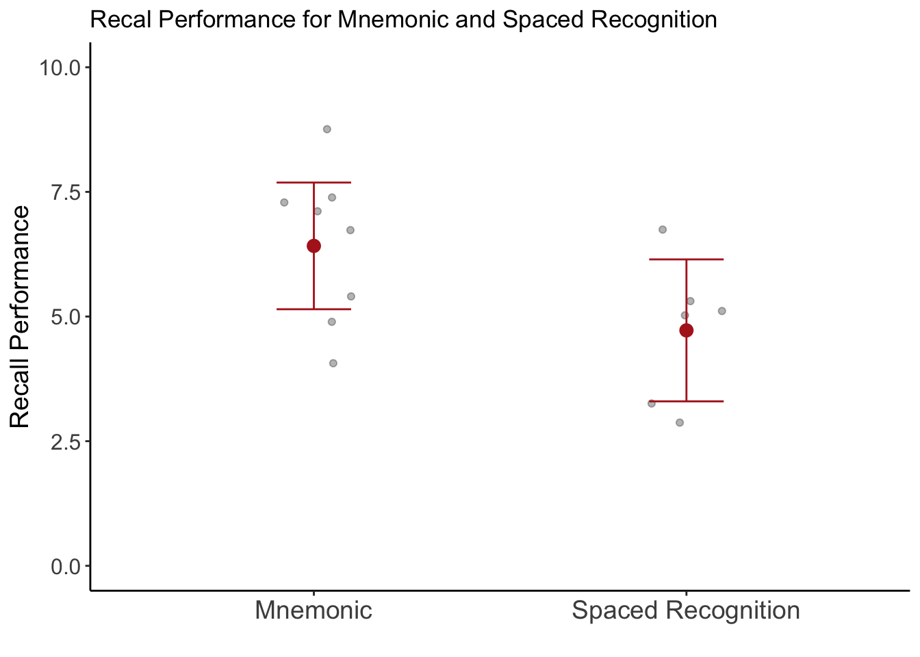
Reproducible Script
Show Code
# load packages
library(readr)
library(dplyr)
library(gt)
library(ggplot2)
# import data
repetition_import <- read_delim("data/class_3_repetition_rawdata.txt",
delim = "\t", escape_double = FALSE,
trim_ws = TRUE)
mnemonic_import <- read_csv("data/class_3_mnemonic_rawdata.csv")
# trasnform data
repetition_data <- repetition_import |>
rename(participant_id = `subject number`,
word_list = List,
recall_correct = recallCorrect) |>
filter(day != "Thursday", day != "Friday") |>
select(participant_id, word_list, recall_correct) |>
mutate(condition = "spaced repetition",
word_list = case_when(word_list == "X" ~ "A",
word_list == "Y" ~ "B",
word_list == "Z" ~ "C")) |>
mutate(.by = word_list,
word_list_mean = mean(recall_correct))
mnemonic_data <- mnemonic_import |>
select(participant_id, condition, word_list, recall_correct)
# merge data
data_merged <- bind_rows(mnemonic_data, repetition_data) |>
  select(-word_list_mean) |>
  arrange(participant_id)
# aggregate data
data_scores <- data_merged |>
  summarise(.by = c(participant_id, condition),
            recall_correct_mean = mean(recall_correct))
# plot aggregate data
ggplot(data_scores, aes(condition, recall_correct_mean)) +
geom_point(position = position_jitter(width = .1, seed = 88), alpha = .3) +
stat_summary(fun = mean, geom = "point",
color = "firebrick", size = 3) +
stat_summary(fun.data = mean_cl_normal, geom = "errorbar",
color = "firebrick", width = .2) +
coord_cartesian(ylim = c(0, 10)) +
scale_x_discrete(labels = c("Mnemonic", "Spaced Recognition")) +
labs(title = "Recal Performance for Mnemonic and Spaced Recognition",
y = "Recall Performance",
x = "") +
theme_classic() +
theme(axis.text.x = element_text(size = 14),
axis.title.y = element_text(size = 14),
axis.text.y = element_text(size = 12))Learning Activity
For this activity we will work with a real data set from a paper published in Psychological Science (one of the top journals in psychology).
Dawtry, R. J., Sutton, R. M., & Sibley, C. G. (2015). Why Wealthier People Think People Are Wealthier, and Why It Matters: From Social Sampling to Attitudes to Redistribution. Psychological Science, 26(9), 1389–1400. https://doi.org/10.1177/0956797615586560
📄 Download the paper (optional)
In this research, Dawtry, Sutton, and Sibley (2015) wanted to examine why people differ in their assessments of the increasing wealth inequality within developed nations. Previous research reveals that most people desire a society in which the overall level of wealth is high and that wealth is spread somewhat equally across society. However, support for this approach to income distribution changes across the social strata. In particular, wealthy people tend to view society as already wealthy and thus are satisfied with the status quo, and less likely to support redistribution. In their paper Dawtry et al., (2015) sought to examine why this is the case. The authors propose that one reason wealthy people tend to view the current system is fair is because their social-circle is comprised of other wealthy people, which biases their perceptions of wealth, which leads them to overestimate the mean level of wealth across society.
To test this hypothesis, the authors conducted a study with 305 participants, recruited from an online participant pool. Participants reported their own annual household income, the income level of those within their own social circle, and the income for the entire population. Participants also rated their perception of the level of equality/inequality across their social circle and across society, their level of satisfaction with and perceived fairness of the current system, their attitudes toward redistribution of wealth (measured using a four-item scale), and their political preference.
Key variables we will look at:
Level of satisfactioin with current system (1 = extremely satisfied, 9 = extremely dissatisfied)
Perceived fairness of current system (1 = extremely fair, 9 = extremely unfair)
Attitude on redistribution of wealth (1 = strongly disagree, 6 = strongly agree)
- contained in four columms:
redist1throughredist4
- contained in four columms:
Political preference (1 = very liberal/very left-wing/strong Democrat, 9 = very conservative/very right-wing/strong Republican):
Political_Preference
Setup
Download the data file
Create a new R script and save it as class3_activity_firstlastname.R
Load the following packages at the top of your script
readr,dplyr,gt,ggplot2
Import the data file
Take some time to explore the data.
- What are the column names?
- What type of values are in the columns?
- How many participants are in the study?
- hint: use a combination of
length()andunique()
- hint: use a combination of
Rename and Filter
Rename the level of satisfaction and perceived fairness columns
In the previous step, you should have noticed how these column names are not ideal. They contain spaces and even a special character
?. You will need to use the special quotation mark` `to reference these column names inrename(), e.g.,`column name with spaces`You can find these special quotation marks to the left of the 1 key and above the tab key.Filter by only keeping rows in which
Political_Preferenceis not missingNA. Note how many fewer rows there are in the data after filtering.hint: use
filter(!is.na())to evaluate whether values inPolitical_Preferenceare NOT!missingis.na()Show cheat code
filter(!is.na(Political_Preference))
Select and Transform
Select only the columns that contain the key variables we are interested in.
Reverse score redist2 and redist4, so that 6=1, 5=2, 4=3, 3=4, 2=5, 1=6.
Use
mutate()andcase_when()Aggregate values across rows
- Calculate a single variable representing participant’s mean attitude on redistrubtion of wealth
- Calculate a single variable representing participant’s mean perception that the current systen is satisfactory and fair.
Use a combination of
rowwise()andmutate()
Summarise
Create a new data frame summarizing the values for attitude on redistribution and the combined satisfactory and fairness variable for each level of political preference. (calculate the mean when summarizing)
Use
summarise(.by = )Create a table of this summarized data frame
Use
gt()from thegtpackage, e.g.,gt(new_data)
Plot
Create a line plot of this summarized data frame
You can copy and paste this, but you might need to change the name of variables to match how you labeled them.
data_summary,redist_mean, andfairnesss_satisfactory_meanggplot(data_summary, aes(Political_Preference)) + geom_line(aes(y = redist_mean, color = "redist")) + geom_line(aes(y = fairness_satisfactory_mean, color = "fair/satis")) + coord_cartesian(xlim = c(1, 9.1), ylim = c(1, 9)) + scale_x_continuous(breaks = 1:9, labels = c("1\nLiberal", "2", "3", "4", "5", "6", "7", "8", "9\nConservative")) + scale_y_continuous(breaks = 1:9, labels = c("Strongly\nDisagree", "2", "3", "4", "5", "6", "7", "8", "Strongly\nAgree")) + scale_color_manual(values = c("redist" = "steelblue", "fair/satis" = "firebrick"), name = "", labels = c("Fairness/Satisfactory of Current System", "Redistribution Preference")) + theme_light() + theme(legend.position = "top") + labs(title = "Economic Attitdues by Political Preference", x = "Political Preference", y = "Attitude")
Check Your Work
You should attempt to complete the activity without looking at this code
Show Code
# load packages
library(readr)
library(dplyr)
library(gt)
library(ggplot2)

# import data
data_import <- read_csv("data/Dawtry Sutton and Sibley 2015 Study 1a.csv")

# data transformation
data <- data_import |>
  rename(fairness = `current system is fair?`,
         satisfactory = `current system is satisfactory?`) |>
  filter(!is.na(Political_Preference)) |>
  select(fairness, satisfactory, redist1, redist2, redist3, redist4,
         Social_Circle_Mean_Income, Political_Preference) |>
  mutate(redist2_recode = case_when(redist2 == 6 ~ 1,
                                    redist2 == 5 ~ 2,
                                    redist2 == 4 ~ 3,
                                    redist2 == 3 ~ 4,
                                    redist2 == 2 ~ 5,
                                    redist2 == 1 ~ 6),
         redist4_recode = case_when(redist4 == 6 ~ 1,
                                    redist4 == 5 ~ 2,
                                    redist4 == 4 ~ 3,
                                    redist4 == 3 ~ 4,
                                    redist4 == 2 ~ 5,
                                    redist4 == 1 ~ 6)) |>
  rowwise() |>
  mutate(redist = mean(c(redist1, redist2, redist3, redist4)),
         fairness_satisfactory = mean(c(fairness, satisfactory))) |>
  ungroup()

# aggregate data
data_summary <- data |>
  summarise(.by = Political_Preference,
            redist_mean = mean(redist),
            fairness_satisfactory_mean = mean(fairness_satisfactory)) |>
  arrange(Political_Preference)

gt(data_summary)

# line plot of summary data
ggplot(data_summary, aes(Political_Preference)) +
  geom_line(aes(y = redist_mean, color = "redist")) +
  geom_line(aes(y = fairness_satisfactory_mean, color = "fair/satis")) +
  coord_cartesian(xlim = c(1, 9), ylim = c(1, 9)) +
  scale_x_continuous(breaks = 1:9,
                     labels =
                       c("1\nLiberal", "2", "3", "4",
                         "5", "6", "7", "8", "9\nConservative")) +
  scale_y_continuous(breaks = 1:9,
                     labels = c("Strongly\nDisagree", "2", "3", "4",
                                "5", "6", "7", "8", "Strongly\nAgree")) +
  scale_color_manual(values = c("redist" = "steelblue",
                                "fair/satis" = "firebrick"),
                     name = "",
                     labels = c("Fairness/Satisfactory of Current System",
                                "Redistribution Preference")) +
  theme_light() +
  theme(legend.position = "top") +
  labs(title = "Economic Attitdues by Political Preference",
       x = "Political Preference",
       y = "Attitude")

ggsave("images/economic_attitudes_by_political_preference.png",
       width = 6, height = 4, dpi = 300)